Ex. 2: \(\mu\)MAG Standard Problem #4
The \(\mu\)MAG project at NIST has proposed a number of micromagnetic standard problems to compare and cross-validate simulation results obtained with different micromagnetic solvers. Here we will simulate the \(\mu\)MAG Standard Problem #4 with tetmag. The simulation will involve several steps already discussed in Example #1, such as the sample geometry definition and the FEM mesh generation, which we won’t repeat here.
This standard problem addresses the magnetization dynamics in a sub-micron sized Permalloy thin-film element during a field-driven magnetic switching process. The sample geometry is a platelet of the size 500 nm \(\times\) 125 nm \(\times\) 3 nm. For the discretization, we will use a FEM cell size of \(3.0\) nm. We start by defining the geometry with FreeCAD, as described in the previous example, and generate a tetrahedral finite-element mesh by using FreeCAD’s netgen plugin.
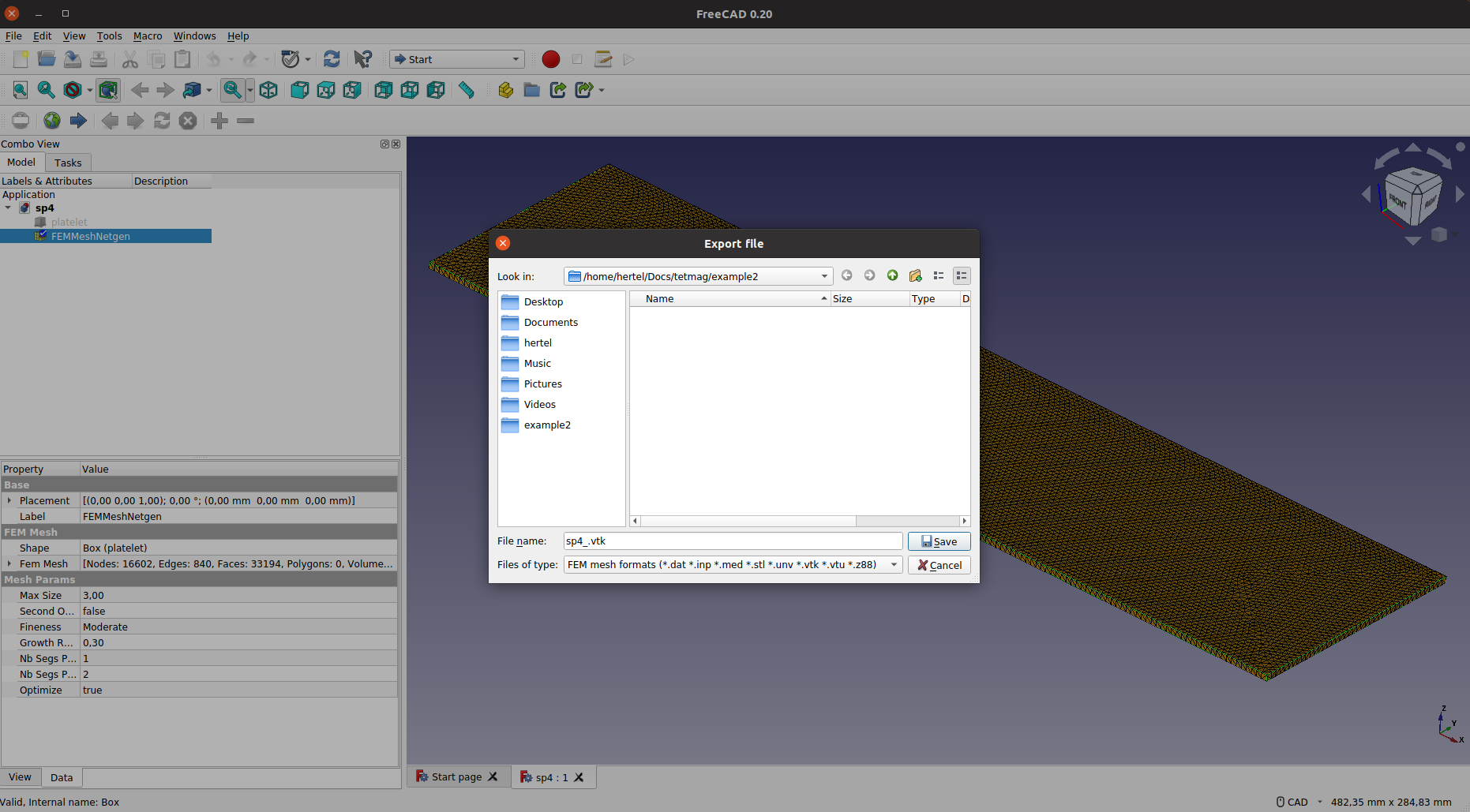
Our mesh contains 48569 tetrahedral elements. We export the FEM mesh file in VTK format. As file name, we choose sp4_.vtk. The underscore is used here to avoid a definition of the <name> ending with a number, which would interfere with the numbered output of VTU files generated during the simulation.
Calculating the initial configuration
The material001.dat file is identical to the one of previous example since, according to the problem specification, the material properties are again those of Permalloy:
A = 1.3e-11
Ms = 8.0e5
The problem specification requires a simulation in two steps. First, a specific zero-field equilibrium configuration, known as “s-state”, is calculated by applying a saturating field along the [1,1,1] direction and gradually reducing it to zero. We will use an external field of \(\mu_0 H=1000\) mT, which we wil reduce in steps of 200 mT to zero. The simulation.cfg file contains the following entries:
name = sp4_
scale = 1.e-9
mesh type = vtk
alpha = 1.0
initial state = homogeneous_x
time step = 0.5 # demag refresh interval in ps
torque limit = 5e-4
duration = 5000  # simulation time in ps
solver type = gpu

hysteresis = yes
  initial field = 1000 # first field value of hysteresis branch, in mT
  final field = 0 # last field of hysteresis branch, in mT
  field step = 200 # step width of increment / decrement in mT
  hys theta = 45 # polar angles of magnetic hysteresis field [deg]
  hys phi = 45 # azimuthal angles of magnetic hysteresis field [deg]

remove precession = yes
The hysteresis keyword indicates that a sequence of equilibrium states will be calculated for different field values, according to the entries in the subsequent lines. The field direction is defined through two angles, theta and phi, of a spherical coordinate system, where theta denotes the angle enclosed between the magnetization and the \(z\) direction, and phi is the angle between the projection of the magnetization on the \(xy\) plane and the \(x\) axis. We use, again, a high damping constant alpha = 1.0 to speed up the calculation and set the keyword remove precession = yes to avoid unwanted precessional magnetization dynamics in this part of the calculation. We choose a somewhat smaller value for the time step than in the previous example to ensure a smooth calcualtion of the magnetization dynamics during the relaxation.
Note
It is strongly recommended to use the option remove precession = yes whenever the hysteresis = yes option is set. Otherwise, the torque limit termination criterion may not be attained during the quasistatic calculation of the magnetization structure.
At the end of this first part of the simulation, we obtain the zero-field “s-state” in the file sp4_.vtu in the working directory. The subdirectory Hysteresis_ contains data on the converged states at the various field steps. We won’t need this data in this project. We rename the VTU file with the s-state configuration to sp4_s-state.vtu, delete all the VTU files with transient states, and the LOG file of the calculation:
mv sp4_.vtu sp4_s-state.vtu
rm sp4_00*vtu sp4_.log
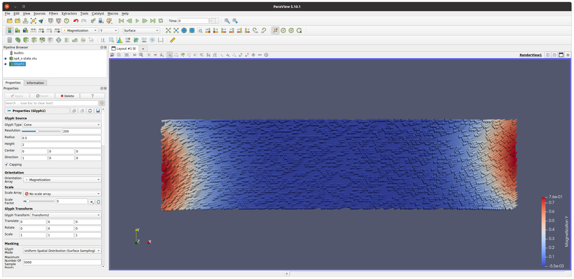
We can verify with ParaView that the configuration is sp4_s-state.vtu contains the expected s-state:
Simulating the switching process
According to the problem specification, a magnetic switching process is initiated by instantanously applying a static magnetic field of 25 mT to the platelet in the s-state configuration, with the field in the \(xy\) plane oriented along a direction enclosing an angle of \(170^\circ\) with the \(x\) axis. Furthermore, the damping constant \(\alpha\) must be set to 0.02.
To use a specific magnetic configuration stored in a VTU file, in our case the s-state from the file sp4_s-state.vtu, as the starting configuration of a simulation, the name of the file must be provided in the initial state entry of the simulation.cfg file, prepended by the expression fromfile_.
The simulation.cfg file used to simulate the field-driven switching contains the following entries:
name = sp4_
scale = 1.e-9
mesh type = vtk
alpha = 0.02
initial state = fromfile_sp4_s-state.vtu
time step = 0.1 # demag refresh interval in ps
duration = 1000  # simulation time in ps
solver type = gpu

external field = 25.0 #  Hext in mT
    theta_H = 90 # polar angle of the field direction in degree
    phi_H = 170 # azimuthal angle
The torque limit entry was removed to ensure that the simulation runs for 1 ns, irrespectice of the evolution of the magnetic structure. Moreover, we lowered the time step value to 0.1 ps, which is genarally a safe choice for low-damping simulations like this one.
The material001.dat file remains unchanged compared to the one used for the quasistatic calculation of the s-state.
After the simulation, the resulting magnetization dynamics can be analyzed as described before. The image below displays the average \(y\) component of the magnetization \(\langle M_y\rangle/M_s\) as a function of time:
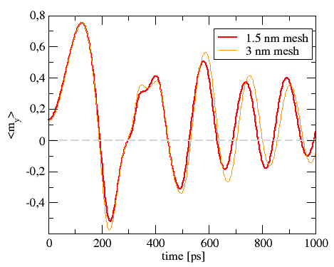
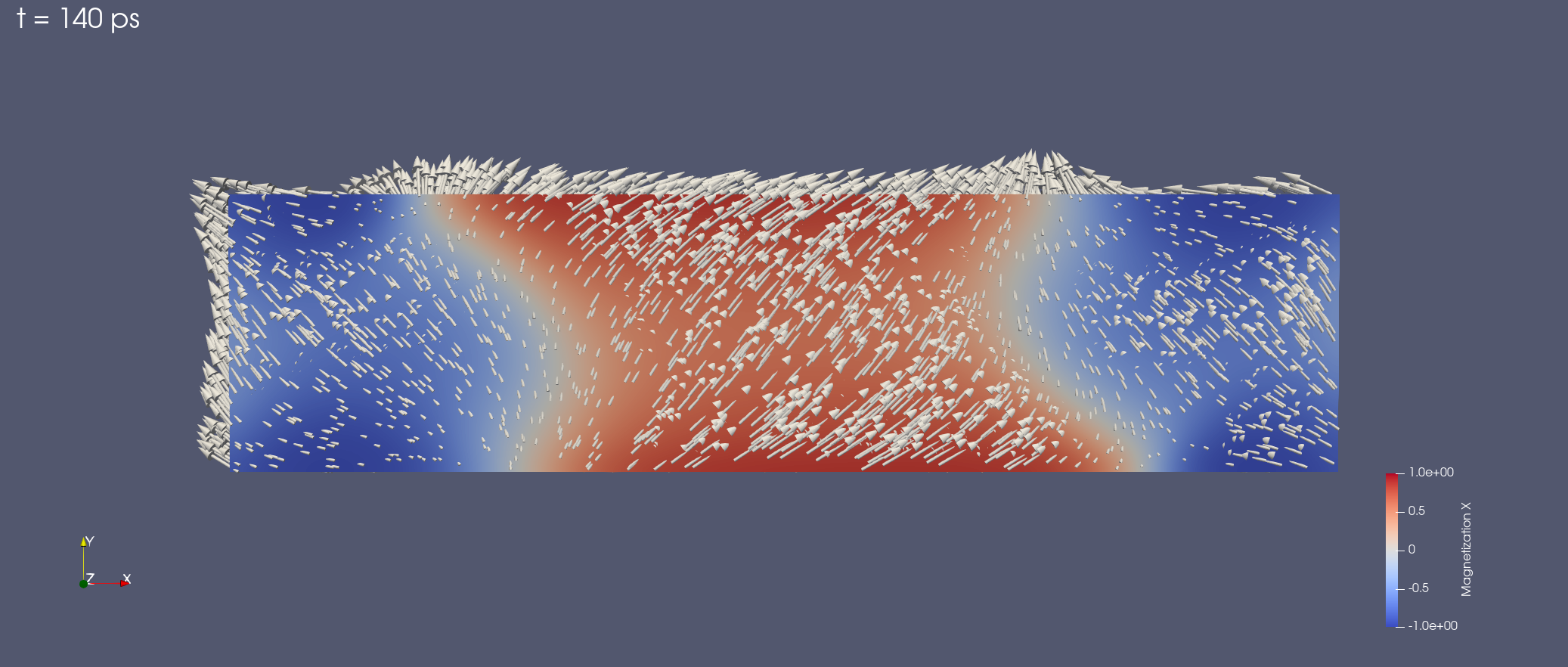
The simulation with the 3 nm mesh yields a result that is already close to that reported by other groups.Better agreement is obtained by lowering the mesh cell size to 1.5 nm. The specification of \(\mu\)MAG Standard Problem #4 requests a representation of a snapshot of the magnetic configuration in the platelet at the moment when the average \(x\) component of the magnetization first crosses the zero line. The value of \(\langle m_x\rangle\) is stored in column #11 of the LOG file. The data shows that the first zero-crossing of \(\langle m_x\rangle\) occurs between \(t=136\) ps and \(t=138\) ps.
  ...
  132.0000        19906.6614      18013.1318      2884.8823       0.0000  -991.3528       0.0000  0.0000  0.0000  3.664e-01       0.08158099865  0.7481174953 -0.1264239146       -0.024620  0.004341  0.000000
  134.0000        19811.6267      18414.0172      3004.6501       0.0000  -1607.0406      0.0000  0.0000  0.0000  3.761e-01       0.04951089997  0.7435191546 -0.1294557353       -0.024620  0.004341  0.000000
  136.0000        19712.4086      18811.0095      3126.6089       0.0000  -2225.2098      0.0000  0.0000  0.0000  3.851e-01       0.01706620831  0.7375109115  -0.132472287       -0.024620  0.004341  0.000000
  138.0000        19608.9898      19203.9153      3249.6787       0.0000  -2844.6042      0.0000  0.0000  0.0000  3.941e-01       -0.01569285578   0.7300725374  -0.1354566535    -0.024620  0.004341  0.000000
  140.0000        19501.3684      19592.6391      3372.7034       0.0000  -3463.9740      0.0000  0.0000  0.0000  4.029e-01       -0.04870499786   0.7211918037  -0.1383929318    -0.024620  0.004341  0.000000
  ...
The closest graphics output we have to this time value is the configuration at \(t=140\) ps: